# install packages
library(ggfortify)
library(ggplot2)
library(caret)
library(MASS)28 Discriminant Analysis - Practical
28.1 Introduction
Before starting this practical, please make sure you have read the previous section and are confident that you understand the key concepts and assumptions behind the approach.
28.2 Linear Discriminant Analysis: Demonstration
Step One: Preparation
We begin by downloading a datafile, and creating a new dataframe lda_data from that file:
lda_data <- read.csv('https://www.dropbox.com/scl/fi/tnbw8s1vbndbfu3zalw4c/lda_01.csv?rlkey=cahnq1v5e197pdv0al1dll99g&dl=1')

lda_data$FavouriteTeam <- NULL
lda_data$X <- NULL
head(lda_data) # display the first six rows
FanGroup Age YearsAsFan MatchesAttended MerchandiseSpending MemberClub
1 Die-Hard 33 8 8 333 Club Z
2 Die-Hard 34 9 5 181 Club Z
3 Die-Hard 43 9 4 107 Club X
4 Die-Hard 39 6 3 227 Club Z
5 Casual 32 3 1 97 Club Y
6 Die-Hard 33 10 8 239 Club XThis dataset contains a range of information gathered from supporters at a rugby match:
Fan Group (Target Variable)
This is the categorical variable we want to predict.
In this case we want to predict whether a supporter belongs to one of two categories -
CasualorDie-Hard.
Remember, we are training our model on data where we already know which of the two categories our participants belong to.
Numerical Variables
Age: Age of the fan.YearsAsFan: Number of years they have been supporting their team.MatchesAttended: Number of rugby matches attended in the last year.MerchandiseSpending: Amount of money spent on merchandise in the last year.
Categorical Variables
MemberClub: Whether they are a member of a rugby fan club (Club X, Y, Z).
Step Two: Data cleaning and preprocessing
It’s vital to ensure that categorical variables are labelled as factors, and handle any missing or outlier values.
lda_data$MemberClub <- as.factor(lda_data$MemberClub)
# Convert target variable to factor if it's not already

lda_data$FanGroup <- as.factor(lda_data$FanGroup) # where 'category' is 'local' or 'visiting' team supporter

# check variables are correctly defined

str(lda_data)
'data.frame': 1000 obs. of 6 variables:
$ FanGroup : Factor w/ 2 levels "Casual","Die-Hard": 2 2 2 2 1 2 1 2 2 2 ...
$ Age : int 33 34 43 39 32 33 25 33 37 39 ...
$ YearsAsFan : int 8 9 9 6 3 10 5 11 11 14 ...
$ MatchesAttended : int 8 5 4 3 1 8 2 4 6 5 ...
$ MerchandiseSpending: int 333 181 107 227 97 239 92 253 238 137 ...
$ MemberClub : Factor w/ 3 levels "Club X","Club Y",..: 3 3 1 3 2 1 3 2 3 3 ...Step Three: Exploratory data analysis
It’s good practice to perform EDA to understand data distributions and relationships. We can visualise the data, focusing on how different variables relate to the target classification.
pairs(lda_data[,1:6], col=lda_data$FanGroup) # Pairwise plots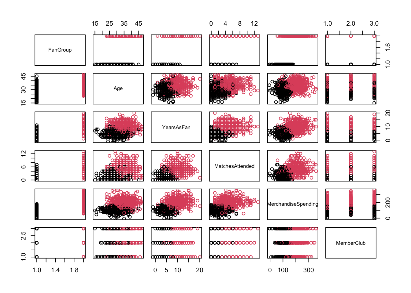
library(ggplot2)

# Boxplot for Age
ggplot(lda_data, aes(x = FanGroup, y = Age, fill = FanGroup)) +
  geom_boxplot() +
  labs(title = "Age by Fan Group", x = "Fan Group", y = "Age")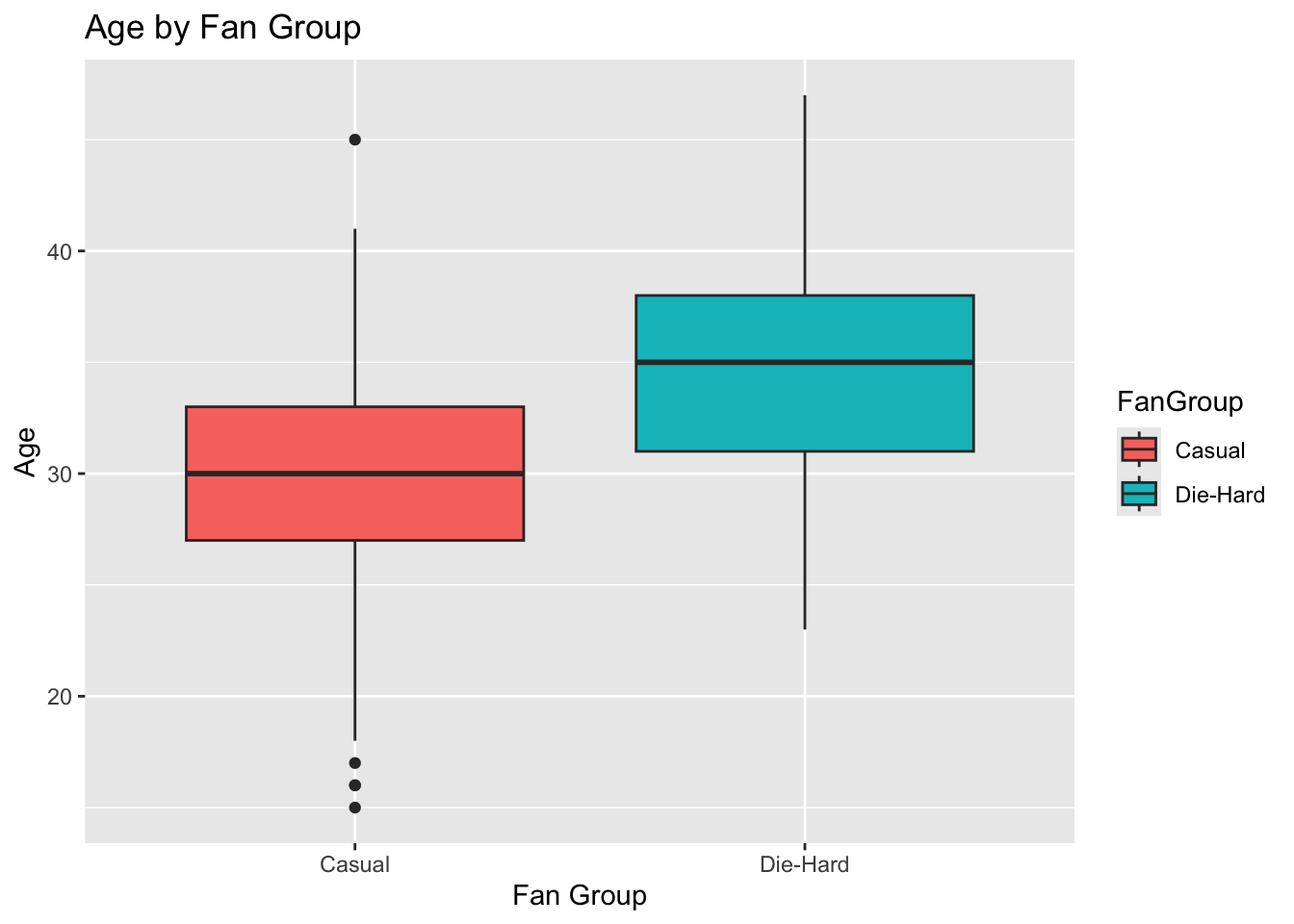
# Boxplot for YearsAsFan
ggplot(lda_data, aes(x = FanGroup, y = YearsAsFan, fill = FanGroup)) +
  geom_boxplot() +
  labs(title = "Years As Fan by Fan Group", x = "Fan Group", y = "Years As Fan")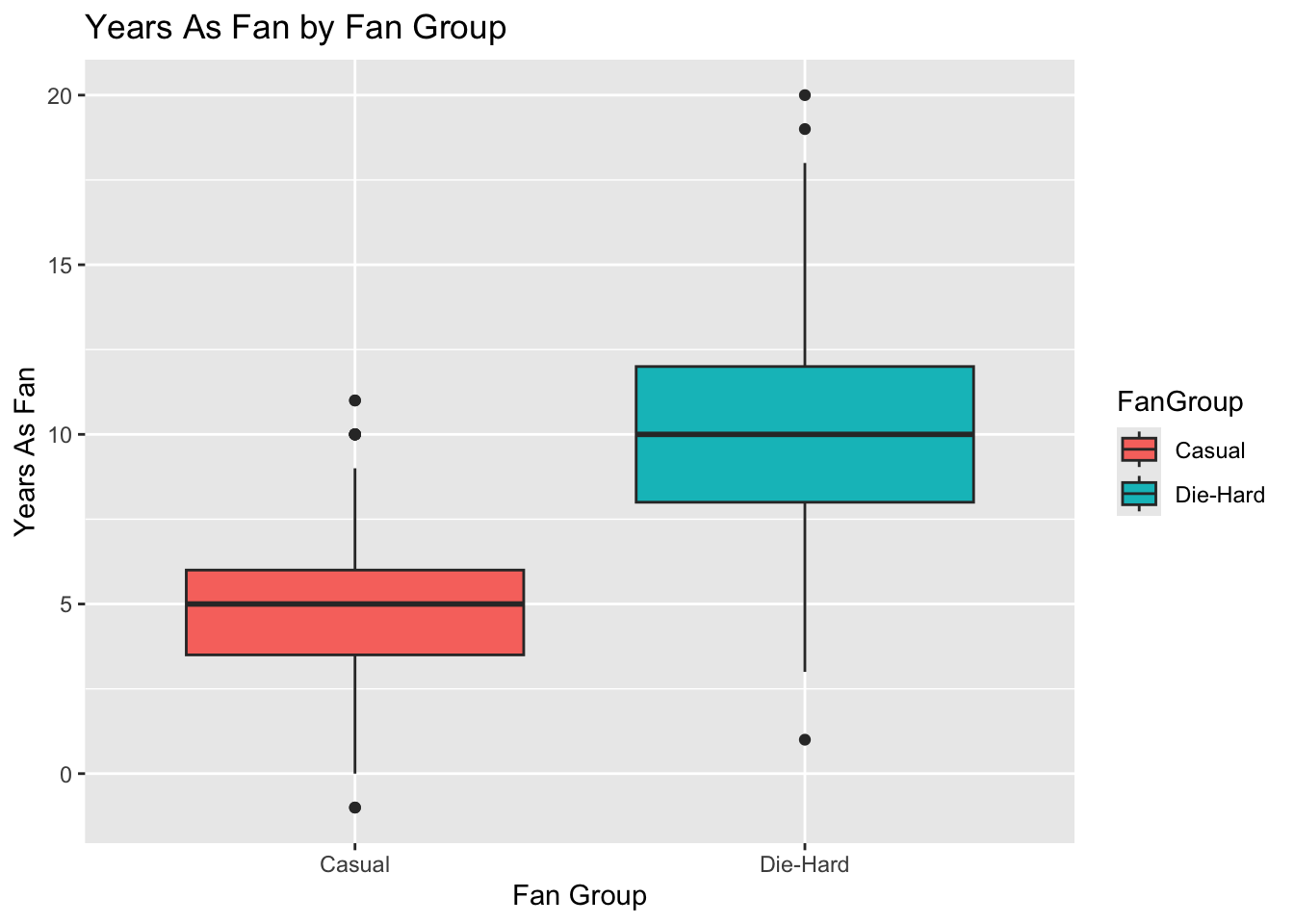
# Boxplot for MatchesAttended
ggplot(lda_data, aes(x = FanGroup, y = MatchesAttended, fill = FanGroup)) +
  geom_boxplot() +
  labs(title = "Matches Attended by Fan Group", x = "Fan Group", y = "Matches Attended")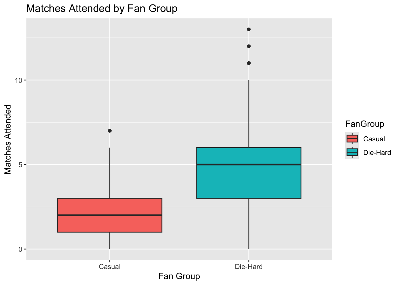
# Boxplot for MerchandiseSpending
ggplot(lda_data, aes(x = FanGroup, y = MerchandiseSpending, fill = FanGroup)) +
  geom_boxplot() +
  labs(title = "Merchandise Spending by Fan Group", x = "Fan Group", y = "Merchandise Spending")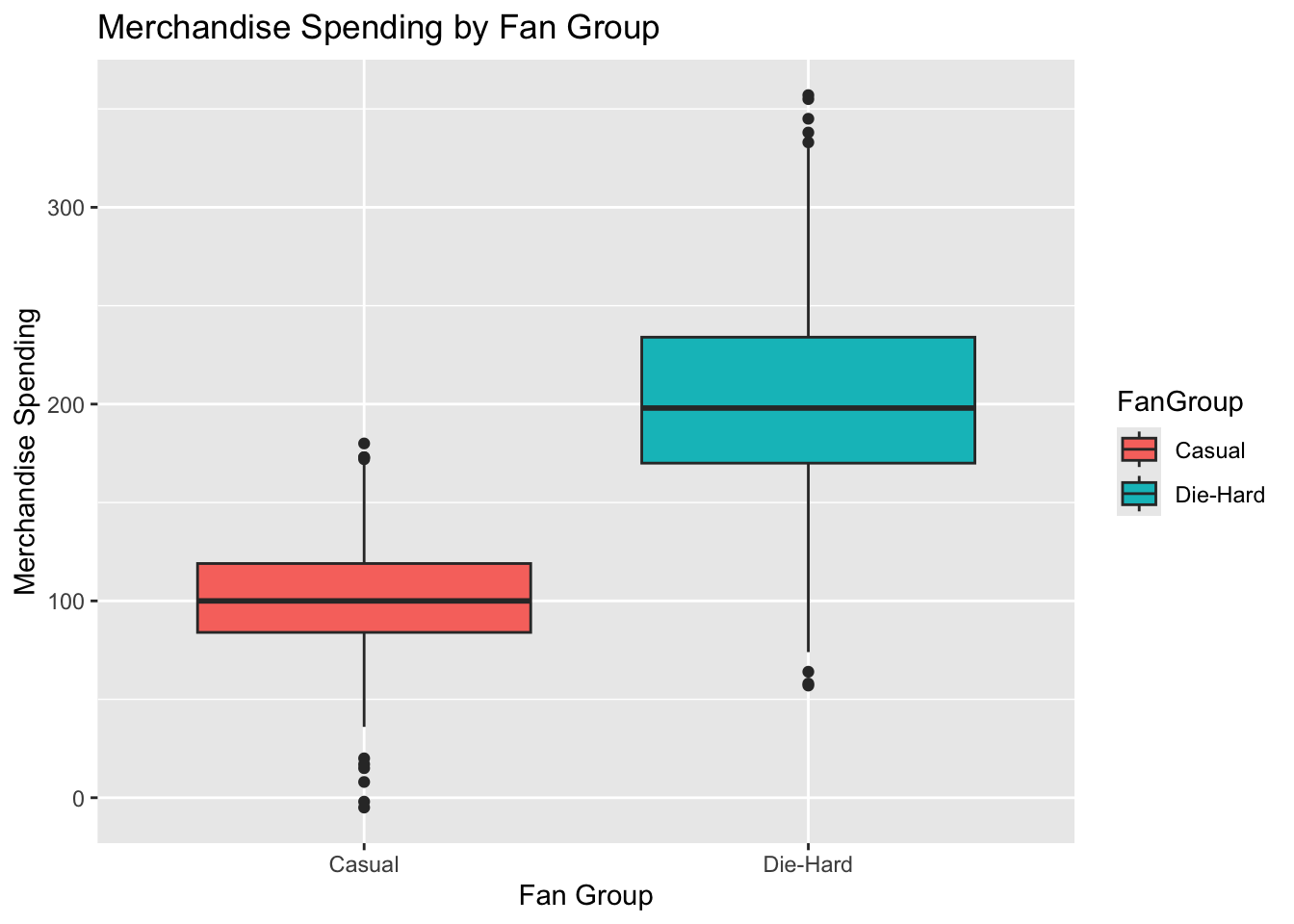
# Bar Plot for MemberClub
ggplot(lda_data, aes(x = MemberClub, fill = FanGroup)) +
  geom_bar(position = "dodge") +
  labs(title = "Member Club by Fan Group", x = "Member Club", y = "Count")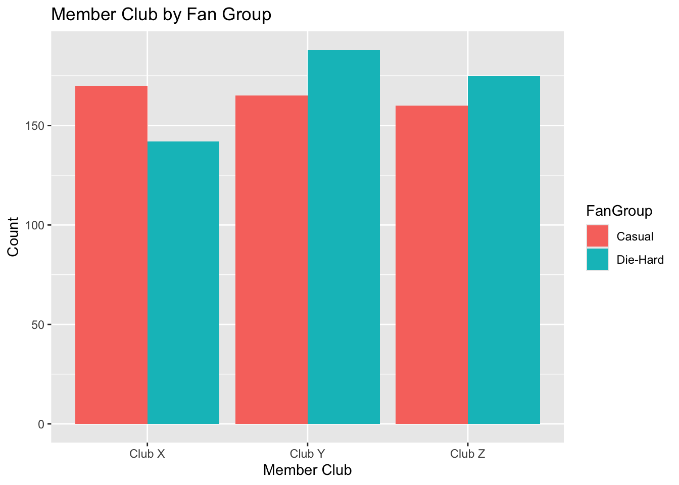
Step Four: Splitting the data
We now divide the data into training and test sets; remember, this will allow us to evaluate the performance of our LDA model by learning with the training set, and checking with the test set.
set.seed(123) # for reproducibility
trainIndex <- sample(1:nrow(lda_data), 0.8 * nrow(lda_data)) # 80% for training
trainData <- lda_data[trainIndex, ]
testData <- lda_data[-trainIndex, ]
In the environment window, you should see that there is a testData dataframe with 200 observations, and a trainData dataframe with 800 observations.
Step Five: Performing LDA
We can use the lda() function from the MASS package to fit the model on the training data.
# note that here, I am manually inputting the variables into the model. later, I will use code that includes ALL variables without having to specify them.

ldaModel <- lda(FanGroup ~ Age + YearsAsFan + MatchesAttended + MerchandiseSpending + MemberClub, data=trainData)

print(ldaModel)
Call:
lda(FanGroup ~ Age + YearsAsFan + MatchesAttended + MerchandiseSpending +
MemberClub, data = trainData)
Prior probabilities of groups:
Casual Die-Hard
0.495 0.505
Group means:
Age YearsAsFan MatchesAttended MerchandiseSpending
Casual 29.99495 4.843434 1.876263 100.5657
Die-Hard 34.94307 10.051980 4.967822 202.0891
MemberClubClub Y MemberClubClub Z
Casual 0.3409091 0.3106061
Die-Hard 0.3366337 0.3688119
Coefficients of linear discriminants:
LD1
Age 0.05610675
YearsAsFan 0.23436786
MatchesAttended 0.20077085
MerchandiseSpending 0.01734080
MemberClubClub Y -0.12424484
MemberClubClub Z -0.02552021Here, we have specified which variables we think might help to predict whether someone is a member of one group (Casual) or the other (Die-Hard). The output suggests that Years as Fan and Matches Attended are the most significant predictive elements in whether someone can be predicted to be a casual or die-hard fan.
Step Six: Model evaluation
We now have a model, and can test the model’s accuracy in predicting whether someone is a casual or die-hard supporter. For this, we use the 20% portion of the original dataset that we retained (testData).
ldaPredict <- predict(ldaModel, testData)
table(ldaPredict$class, testData$FanGroup)
           Casual Die-Hard
  Casual       97        3
  Die-Hard      2       98
# Calculate accuracy
mean(ldaPredict$class == testData$FanGroup)[1] 0.975This suggests that our model is very good at prediction…it predicts the correct category 98% of the time.
Step Seven: Diagnostics and interpretation
Finally, we evaluate the model coefficients and the confusion matrix to understand the influence of each variable.
Note that, because we only have two different outcome groups, there is only one Linear Discriminant (LD) in this model.
ldaModel$scaling LD1
Age 0.05610675
YearsAsFan 0.23436786
MatchesAttended 0.20077085
MerchandiseSpending 0.01734080
MemberClubClub Y -0.12424484
MemberClubClub Z -0.02552021# Confusion Matrix
confusionMatrix(ldaPredict$class, testData$FanGroup)Confusion Matrix and Statistics
Reference
Prediction Casual Die-Hard
Casual 97 3
Die-Hard 2 98
Accuracy : 0.975
95% CI : (0.9426, 0.9918)
No Information Rate : 0.505
P-Value [Acc > NIR] : <2e-16
Kappa : 0.95
Mcnemar's Test P-Value : 1
Sensitivity : 0.9798
Specificity : 0.9703
Pos Pred Value : 0.9700
Neg Pred Value : 0.9800
Prevalence : 0.4950
Detection Rate : 0.4850
Detection Prevalence : 0.5000
Balanced Accuracy : 0.9750
'Positive' Class : Casual
print(confusionMatrix)function (data, ...)
{
UseMethod("confusionMatrix")
}
<bytecode: 0x7f994faa9570>
<environment: namespace:caret>We can also plot the outcome of the model:
lda_model <- lda(FanGroup ~ ., data = lda_data)

# Predict using the LDA model
lda_pred <- predict(lda_model)

# Add LDA components to the original data
lda_model <- cbind(lda_data, lda_pred$x)

# LDA Component 1 by Species
ggplot(lda_model, aes(FanGroup, LD1, fill = FanGroup)) +
  geom_boxplot() +
  ggtitle("Boxplot of LD1 by Species")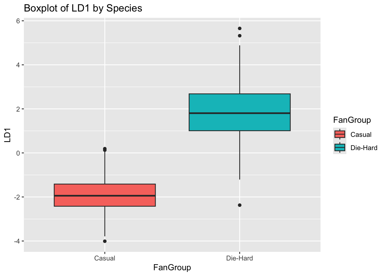
28.3 Linear Discriminant Analysis: Practice
Now, using the following dataset, repeat Steps 1-7 listed above.
# Step One: Load Dataset

lda_data_02 <- read.csv('https://www.dropbox.com/scl/fi/p4hr96dtpgii50ufbn8oo/lda_02.csv?rlkey=jx7we1wggbb4n6xm8bqrllvay&dl=1')

head(lda_data_02) # display the first six rows
X FanGroup Age YearsAsFan MatchesAttended MerchandiseSpending FavouriteTeam
1 1 Regular 24 3 4 173 Team D
2 2 Casual 20 4 6 229 Team A
3 3 Casual 40 2 3 131 Team C
4 4 Die-Hard 38 7 9 131 Team J
5 5 Die-Hard 15 8 13 182 Team H
6 6 Regular 29 11 6 102 Team G
MemberClub SocialMediaEngagement
1 Club 1 57
2 Club 1 21
3 Club 1 33
4 Club 3 88
5 Club 1 88
6 Club 4 42Show code for Step Two Data Cleaning and Preprocessing
###----------------------------------------------
### Step Two: Data cleaning and preprocessing

# get rid of old stuff in environment

rm(lda_data, lda_model, lda_pred, ldaModel, ldaPredict, testData, trainData)

lda_data_02$MemberClub <- as.factor(lda_data_02$MemberClub)

# Convert target variable to factor if it's not already

lda_data_02$FanGroup <- as.factor(lda_data_02$FanGroup) # where 'category' is regular/casual/die-hard

# check variables are correctly defined

str(lda_data_02)
Show code for Step Three Exploratory data analysis
###----------------------------------------------
### Step Three: Exploratory data analysis

pairs(lda_data_02[,1:6], col=lda_data_02$FanGroup)  # Pairwise plots

library(ggplot2)

# Boxplot for Age
ggplot(lda_data_02, aes(x = FanGroup, y = Age, fill = FanGroup)) +
  geom_boxplot() +
  labs(title = "Age by Fan Group", x = "Fan Group", y = "Age")

# Boxplot for YearsAsFan
ggplot(lda_data_02, aes(x = FanGroup, y = YearsAsFan, fill = FanGroup)) +
  geom_boxplot() +
  labs(title = "Years As Fan by Fan Group", x = "Fan Group", y = "Years As Fan")

# Boxplot for MatchesAttended
ggplot(lda_data_02, aes(x = FanGroup, y = MatchesAttended, fill = FanGroup)) +
  geom_boxplot() +
  labs(title = "Matches Attended by Fan Group", x = "Fan Group", y = "Matches Attended")

# Boxplot for MerchandiseSpending
ggplot(lda_data_02, aes(x = FanGroup, y = MerchandiseSpending, fill = FanGroup)) +
  geom_boxplot() +
  labs(title = "Merchandise Spending by Fan Group", x = "Fan Group", y = "Merchandise Spending")

# Boxplot for SocialMediaEngagement
ggplot(lda_data_02, aes(x = FanGroup, y = SocialMediaEngagement, fill = FanGroup)) +
  geom_boxplot() +
  labs(title = "Social Media Engagement by Fan Group", x = "Fan Group", y = "Social Media Engagement")

# Bar Plot for MemberClub
ggplot(lda_data_02, aes(x = MemberClub, fill = FanGroup)) +
  geom_bar(position = "dodge") +
  labs(title = "Member Club by Fan Group", x = "Member Club", y = "Count")
Show code for Step Four Splitting the data
###----------------------------------------------
### Step Four: Splitting the data

set.seed(123) # for reproducibility
trainIndex <- sample(1:nrow(lda_data_02), 0.8 * nrow(lda_data_02)) # 80% for training
trainData_02 <- lda_data_02[trainIndex, ]
testData_02 <- lda_data_02[-trainIndex, ]
Show code for Step Five Performing LDA
###----------------------------------------------
### Step Five: Performing LDA

ldaModel_02 <- lda(FanGroup ~ Age + YearsAsFan + MatchesAttended + MerchandiseSpending + SocialMediaEngagement + MemberClub, data=trainData_02)

print(ldaModel_02)
Show code for Step Six Model evaluation
###----------------------------------------------
### Step Six: Model evaluation

ldaPredict <- predict(ldaModel_02, testData_02)
table(ldaPredict$class, testData_02$FanGroup)

# Calculate accuracy
mean(ldaPredict$class == testData_02$FanGroup)
Show code for Step Seven Diagnostics and interpretation
###----------------------------------------------
### Step Seven: Diagnostics and interpretation

library(ggplot2)

ldaModel_02$scaling
# Confusion Matrix

confusionMatrix(ldaPredict$class,testData_02$FanGroup)
print(confusionMatrix)


# Add LDA components to the original data
lda_data_02 <- cbind(lda_data_02, ldaPredict$x)

# LDA Component 1 by Species
ggplot(lda_data_02, aes(FanGroup, LD1, fill = FanGroup)) +
  geom_boxplot() +
  ggtitle("Boxplot of LD1 by Species")
Show code for Step Seven Diagnostics and interpretation
# LDA Component 2 by Species
ggplot(lda_data_02, aes(FanGroup, LD2, fill = FanGroup)) +
  geom_boxplot() +
  ggtitle("Boxplot of LD2 by Species")
28.4 Walk-Through: Quadratic Discriminant Analysis
Introduction
The value of a QDA (rather than an LDA) is that it can cope with situations where our variables have different distribution shapes, as well as different means.
The basic process for analysis is the same as for LDA.
In this example, I have a dataset that contains a range of player attributes. I am trying to develop a model that will help me predict which position a player plays, based on those attributes.
Show code for synthetic data generation
set.seed(123) # for reproducibility

# Number of observations
n <- 500

# Generate data
Position <- sample(c("Goalkeeper", "Defender", "Midfielder", "Forward"), n, replace = TRUE)
Age <- round(runif(n, 12, 18)) # Ages 12 to 18
Height <- round(rnorm(n, mean = 160, sd = 10)) # Height in cm
Weight <- round(rnorm(n, mean = 55, sd = 15)) # Weight in kg
Speed <- round(rnorm(n, mean = 50, sd = 10)) # Speed, arbitrary units
Stamina <- round(rnorm(n, mean = 50, sd = 10)) # Stamina, arbitrary units
PassingAccuracy <- ifelse(Position == "Midfielder" | Position == "Forward", round(rnorm(n, 60, 10)), round(rnorm(n, 40, 10)))
TacklingAbility <- ifelse(Position == "Defender", round(rnorm(n, 60, 10)), round(rnorm(n, 40, 10)))
GoalScoringRecord <- ifelse(Position == "Forward", round(rnorm(n, 6, 2)), round(rnorm(n, 2, 1))) # Goals per season

# Create the data frame
df_soccer <- data.frame(Position, Age, Height, Weight, Speed, Stamina, PassingAccuracy, TacklingAbility, GoalScoringRecord)


df_soccer$Position <- as.factor(df_soccer$Position)

# View the first few rows of the dataframe
head(df_soccer)
First, I’ll load the required libraries for analysis:
library(MASS)Then, I’ll prepare the dataset by splitting it into training and testing datasets:
set.seed(123)  # for reproducibility

# I'm going to split my dataset into two parts, with 75% being used for training, and 25% being kept back for testing

split_index <- sample(1:nrow(df_soccer), nrow(df_soccer)*0.7)

train_data <- df_soccer[split_index, ]
test_data <- df_soccer[-split_index, ]
To conduct the QDA, I’ll use the qda function from the MASS package. In this case, I’m going to put all of the variables into the model.
qda_model <- qda(Position ~ ., data = train_data)Then, I can make predictions on the test dataset, based on the output from my qda model:
qda_predictions <- predict(qda_model, test_data)
print(qda_predictions)
$class
[1] Midfielder Midfielder Defender Defender Goalkeeper Goalkeeper
[7] Goalkeeper Forward Goalkeeper Forward Goalkeeper Forward
[13] Midfielder Midfielder Defender Goalkeeper Defender Midfielder
[19] Goalkeeper Goalkeeper Midfielder Goalkeeper Goalkeeper Forward
[25] Forward Goalkeeper Goalkeeper Goalkeeper Midfielder Forward
[31] Defender Forward Goalkeeper Goalkeeper Midfielder Defender
[37] Defender Midfielder Goalkeeper Defender Midfielder Goalkeeper
[43] Goalkeeper Midfielder Forward Midfielder Defender Defender
[49] Forward Goalkeeper Defender Forward Defender Midfielder
[55] Midfielder Goalkeeper Midfielder Goalkeeper Goalkeeper Midfielder
[61] Forward Goalkeeper Midfielder Defender Goalkeeper Defender
[67] Goalkeeper Goalkeeper Goalkeeper Forward Midfielder Forward
[73] Defender Goalkeeper Defender Midfielder Forward Midfielder
[79] Forward Forward Midfielder Defender Defender Goalkeeper
[85] Defender Goalkeeper Midfielder Goalkeeper Midfielder Goalkeeper
[91] Goalkeeper Goalkeeper Defender Defender Goalkeeper Forward
[97] Goalkeeper Defender Goalkeeper Forward Midfielder Goalkeeper
[103] Defender Forward Midfielder Midfielder Forward Defender
[109] Defender Midfielder Forward Goalkeeper Defender Defender
[115] Forward Goalkeeper Goalkeeper Goalkeeper Midfielder Defender
[121] Goalkeeper Goalkeeper Goalkeeper Goalkeeper Forward Forward
[127] Goalkeeper Goalkeeper Defender Goalkeeper Goalkeeper Defender
[133] Defender Forward Forward Midfielder Goalkeeper Goalkeeper
[139] Midfielder Midfielder Midfielder Defender Defender Forward
[145] Forward Midfielder Forward Midfielder Midfielder Midfielder
Levels: Defender Forward Goalkeeper Midfielder
$posterior
Defender Forward Goalkeeper Midfielder
1 4.610490e-02 1.483206e-02 2.871579e-01 6.519052e-01
3 3.262841e-01 7.455396e-03 2.607025e-01 4.055580e-01
6 8.746858e-01 6.189967e-04 1.196205e-01 5.074655e-03
8 8.729758e-01 6.570172e-05 1.268928e-01 6.571052e-05
9 6.632356e-03 1.078914e-01 6.711852e-01 2.142911e-01
12 1.012115e-01 4.757631e-04 8.983095e-01 3.190509e-06
15 6.667185e-02 2.424110e-03 7.520111e-01 1.788929e-01
17 3.761390e-08 9.999984e-01 6.159712e-07 9.498238e-07
18 7.773372e-03 3.753135e-02 6.177525e-01 3.369428e-01
19 6.449722e-03 9.420601e-01 1.383425e-02 3.765588e-02
28 3.274642e-01 2.128057e-04 6.722828e-01 4.015963e-05
29 6.068279e-04 5.647200e-01 9.758911e-02 3.370840e-01
37 1.527443e-01 2.857018e-02 5.321721e-02 7.654683e-01
38 2.759259e-02 6.492798e-02 3.412147e-01 5.662647e-01
44 5.826901e-01 6.420046e-02 2.315212e-01 1.215883e-01
46 1.033869e-03 1.325828e-03 9.965923e-01 1.048041e-03
47 5.614573e-01 4.741034e-03 4.001430e-01 3.365867e-02
49 1.814379e-03 3.282631e-01 2.040454e-03 6.678821e-01
50 5.033831e-02 3.190912e-03 7.421402e-01 2.043306e-01
56 1.746069e-02 5.245143e-02 8.710477e-01 5.904018e-02
58 1.839648e-03 2.156415e-01 1.605087e-01 6.220102e-01
59 4.859555e-01 2.978761e-04 5.105068e-01 3.239831e-03
60 3.554547e-01 3.933357e-03 6.318857e-01 8.726164e-03
62 4.964813e-12 9.999998e-01 4.142570e-10 1.653235e-07
65 5.268420e-03 7.177488e-01 9.314552e-02 1.838372e-01
68 1.603385e-02 3.835953e-02 5.666799e-01 3.789267e-01
70 1.078367e-01 6.890769e-03 7.809492e-01 1.043233e-01
71 4.764484e-01 3.188904e-04 5.120099e-01 1.122277e-02
75 1.776141e-01 2.221677e-03 2.713871e-01 5.487771e-01
79 2.717634e-08 9.999990e-01 8.457890e-07 1.393324e-07
88 9.381216e-01 1.931247e-05 6.047074e-02 1.388384e-03
95 1.469771e-08 9.999982e-01 1.052299e-08 1.819049e-06
97 7.822327e-03 8.192046e-03 9.646724e-01 1.931319e-02
99 9.975099e-02 8.976188e-03 8.234160e-01 6.785686e-02
100 6.152702e-03 6.009827e-02 4.066079e-03 9.296829e-01
101 4.631280e-01 1.336384e-02 3.320308e-01 1.914774e-01
103 7.343629e-01 1.000489e-02 2.256671e-01 2.996507e-02
108 2.859027e-02 5.560684e-03 4.666818e-01 4.991672e-01
114 1.603062e-02 7.895576e-03 7.617989e-01 2.142749e-01
120 8.354422e-01 6.269823e-04 1.486123e-01 1.531845e-02
123 1.013483e-03 4.446630e-02 2.253674e-04 9.542949e-01
124 6.091421e-02 4.333754e-02 5.400985e-01 3.556497e-01
126 2.026759e-01 2.538424e-03 7.845185e-01 1.026718e-02
128 3.480691e-04 7.069479e-03 5.339632e-02 9.391861e-01
131 6.569078e-14 1.000000e+00 2.773709e-10 4.245321e-15
132 8.832516e-04 7.892408e-04 3.456426e-02 9.637632e-01
138 9.130922e-01 1.361321e-05 8.364409e-02 3.250121e-03
139 5.125825e-01 3.025931e-04 4.843915e-01 2.723387e-03
142 2.616026e-05 9.948798e-01 1.901482e-04 4.903867e-03
144 7.888531e-02 1.990777e-03 9.110694e-01 8.054545e-03
147 9.273009e-01 1.776124e-05 6.911919e-02 3.562181e-03
149 4.763986e-06 9.993554e-01 3.027217e-05 6.095706e-04
150 6.653197e-01 1.733272e-03 2.705840e-01 6.236305e-02
156 1.231593e-03 4.429367e-03 8.936313e-02 9.049759e-01
157 1.256861e-01 3.702676e-03 1.535136e-02 8.552599e-01
162 2.091077e-01 5.031980e-03 7.593095e-01 2.655085e-02
167 5.874204e-04 2.925977e-02 2.741022e-02 9.427426e-01
169 1.994879e-01 1.674029e-01 5.926906e-01 4.041861e-02
175 1.442287e-01 5.086939e-04 8.398925e-01 1.537003e-02
180 1.891926e-01 7.580183e-02 3.889173e-02 6.961138e-01
181 1.160833e-07 9.999955e-01 4.144117e-06 2.696242e-07
182 3.994123e-02 1.083617e-01 5.534091e-01 2.982880e-01
183 3.511311e-02 7.613890e-03 1.592845e-01 7.979885e-01
187 7.795368e-01 2.754148e-04 2.195151e-01 6.726101e-04
188 4.019442e-01 4.787915e-03 5.729177e-01 2.035011e-02
190 7.342039e-01 1.559522e-03 2.426427e-01 2.159384e-02
193 2.220509e-01 1.685019e-01 3.313840e-01 2.780633e-01
203 8.368558e-02 9.408502e-03 9.062114e-01 6.944788e-04
204 1.510597e-04 1.422590e-01 7.690223e-01 8.856764e-02
206 9.874701e-03 5.030215e-01 3.897202e-02 4.481318e-01
208 1.550086e-01 9.642229e-02 1.259999e-01 6.225692e-01
216 5.677513e-05 9.657602e-01 1.134038e-03 3.304900e-02
219 6.871400e-01 1.408137e-03 2.414832e-01 6.996871e-02
231 2.956624e-02 1.869480e-02 9.092733e-01 4.246563e-02
233 7.056395e-01 4.261438e-04 2.886620e-01 5.272359e-03
237 8.184035e-04 3.670689e-01 1.417441e-04 6.319709e-01
239 1.503498e-06 9.998830e-01 8.999597e-05 2.547185e-05
246 9.280960e-02 4.758198e-04 1.003879e-01 8.063267e-01
247 1.087658e-02 4.959268e-01 4.152442e-01 7.795246e-02
248 1.095932e-06 9.999756e-01 2.334950e-05 1.434104e-09
258 8.640372e-04 3.986575e-01 5.323932e-04 5.999461e-01
259 9.911538e-01 2.313809e-07 8.839496e-03 6.440849e-06
269 6.026727e-01 6.053770e-04 3.575466e-01 3.917529e-02
271 3.612357e-02 3.878522e-04 9.147338e-01 4.875474e-02
274 7.932840e-01 2.040362e-04 2.010658e-01 5.446178e-03
276 2.291589e-01 3.938992e-03 7.285351e-01 3.836699e-02
283 2.103155e-01 1.979916e-02 6.209498e-03 7.636758e-01
293 4.910177e-02 4.857955e-03 8.646019e-01 8.143838e-02
295 3.354893e-02 4.604304e-02 5.458156e-02 8.658265e-01
300 3.946256e-01 9.867904e-04 5.857397e-01 1.864794e-02
303 1.766396e-01 8.094643e-02 3.854677e-01 3.569462e-01
312 9.047702e-02 8.201295e-03 7.041482e-01 1.971735e-01
317 9.327166e-01 1.899615e-05 6.688983e-02 3.746063e-04
323 7.538815e-01 1.403228e-05 2.461023e-01 2.116861e-06
324 1.879451e-01 5.560941e-03 7.756722e-01 3.082179e-02
325 1.018776e-09 9.999990e-01 7.006571e-08 9.759268e-07
333 1.583243e-02 2.469188e-03 8.474589e-01 1.342395e-01
334 4.004566e-01 3.788420e-03 2.936270e-01 3.021280e-01
336 3.079168e-02 9.073701e-03 9.326727e-01 2.746192e-02
337 4.228774e-08 9.999801e-01 1.784986e-05 1.996505e-06
338 8.851595e-04 5.754056e-02 9.888519e-02 8.426891e-01
341 7.132497e-02 7.793430e-03 8.138501e-01 1.070315e-01
345 6.698654e-01 8.926278e-03 2.800275e-01 4.118089e-02
349 3.174965e-05 9.993834e-01 1.798551e-04 4.049615e-04
354 4.299850e-01 9.043455e-04 7.367636e-03 5.617430e-01
358 8.025265e-03 2.084861e-01 4.125322e-02 7.422354e-01
360 1.677598e-07 9.985071e-01 2.193972e-05 1.470830e-03
365 9.816349e-01 1.065777e-06 1.813602e-02 2.279845e-04
367 7.797494e-01 3.814713e-04 2.196248e-01 2.443846e-04
371 3.027386e-04 1.464664e-01 4.937486e-04 8.527371e-01
377 3.731130e-11 1.000000e+00 2.358181e-11 5.385208e-11
379 9.799031e-02 2.778956e-02 8.240098e-01 5.021034e-02
380 4.951032e-01 2.522294e-03 7.349865e-02 4.288759e-01
385 8.698710e-01 1.589812e-04 1.201106e-01 9.859370e-03
387 2.421189e-10 1.000000e+00 1.269926e-08 9.582166e-11
398 2.132352e-02 1.902351e-01 4.188917e-01 3.695497e-01
404 4.923771e-03 1.480071e-02 9.553326e-01 2.494294e-02
406 4.321554e-03 1.480384e-01 6.717002e-01 1.759399e-01
408 1.637788e-03 1.052518e-04 4.382580e-04 9.978187e-01
412 9.257897e-01 2.598889e-05 7.413264e-02 5.165602e-05
416 2.218674e-02 1.863964e-03 9.516466e-01 2.430271e-02
418 2.796958e-02 1.135539e-02 8.078078e-01 1.528673e-01
419 1.092781e-01 3.477151e-01 5.269273e-01 1.607946e-02
423 4.275837e-01 1.230855e-02 5.300416e-01 3.006609e-02
427 1.542209e-02 9.478879e-01 3.406600e-02 2.624002e-03
432 3.052320e-02 9.490274e-01 2.043409e-02 1.528961e-05
435 8.455924e-02 3.334256e-03 9.004152e-01 1.169132e-02
436 1.427119e-01 2.054726e-02 8.185721e-01 1.816882e-02
443 9.482966e-01 1.829839e-04 5.102657e-02 4.938585e-04
445 7.927878e-02 1.879784e-02 7.402118e-01 1.617116e-01
448 4.764083e-03 2.531843e-02 5.760081e-01 3.939094e-01
449 8.000372e-01 2.455925e-04 1.994094e-01 3.078011e-04
451 8.285835e-01 8.947833e-04 1.517905e-01 1.873123e-02
460 1.656566e-14 1.000000e+00 2.918711e-14 3.042814e-11
461 2.010423e-04 9.605116e-01 2.476724e-03 3.681059e-02
462 3.582181e-01 2.446875e-02 7.632025e-03 6.096812e-01
464 3.159069e-02 2.796765e-01 3.464604e-01 3.422724e-01
465 7.319143e-02 2.973531e-03 7.995348e-01 1.243003e-01
468 1.814967e-03 3.666316e-01 1.641329e-01 4.674206e-01
470 2.014716e-02 2.718412e-02 1.035166e-01 8.491521e-01
471 1.679297e-03 2.057259e-02 7.118272e-05 9.776769e-01
482 8.323214e-01 4.641476e-05 1.562282e-01 1.140398e-02
483 9.517474e-01 1.054461e-06 4.822017e-02 3.135386e-05
484 4.361179e-17 1.000000e+00 6.307301e-14 2.341099e-19
489 8.536195e-09 1.000000e+00 1.011102e-08 7.045152e-15
490 3.026212e-02 1.763200e-01 2.613529e-03 7.908043e-01
492 2.095462e-04 9.993655e-01 4.249422e-04 1.461261e-08
498 1.682647e-01 9.255035e-02 3.260368e-01 4.131482e-01
499 4.643480e-04 1.833264e-01 5.470921e-03 8.107383e-01
500 7.177852e-03 5.030371e-02 1.711676e-01 7.713508e-01Now, I can evaluate the model using a confusion matrix, to see how well my model performed in terms of its predictions:
confusionMatrix(qda_predictions$class, test_data$Position)Confusion Matrix and Statistics
Reference
Prediction Defender Forward Goalkeeper Midfielder
Defender 26 0 6 1
Forward 0 25 2 2
Goalkeeper 10 3 30 9
Midfielder 1 2 3 30
Overall Statistics
Accuracy : 0.74
95% CI : (0.6621, 0.8081)
No Information Rate : 0.28
P-Value [Acc > NIR] : < 2.2e-16
Kappa : 0.6511
Mcnemar's Test P-Value : NA
Statistics by Class:
Class: Defender Class: Forward Class: Goalkeeper
Sensitivity 0.7027 0.8333 0.7317
Specificity 0.9381 0.9667 0.7982
Pos Pred Value 0.7879 0.8621 0.5769
Neg Pred Value 0.9060 0.9587 0.8878
Prevalence 0.2467 0.2000 0.2733
Detection Rate 0.1733 0.1667 0.2000
Detection Prevalence 0.2200 0.1933 0.3467
Balanced Accuracy 0.8204 0.9000 0.7649
Class: Midfielder
Sensitivity 0.7143
Specificity 0.9444
Pos Pred Value 0.8333
Neg Pred Value 0.8947
Prevalence 0.2800
Detection Rate 0.2000
Detection Prevalence 0.2400
Balanced Accuracy 0.8294To finish, I’ll look at calculating the overall accuracy of my model:
accuracy <- mean(qda_predictions$class == test_data$Position)
print(paste("Accuracy:", accuracy))
[1] "Accuracy: 0.74"28.5 Your Turn: Quadratic Discriminant Analysis
Repeat the steps above.
Experiment with the dataset: what happens when you remove variables from the model? Does the model accuracy improve, or deteriorate?
Extension task: how can we evaluate the importance of the different variables in the predictive accuracy of our model? In other words, what would we do with the model once we know it’s accurate?